8 Canonical Correlation
In this chapter we introduce the concept of canonical correlation and explore some of the ways this method can help us unpack the relationships that exist between sets of variables, rather than between individual variables themselves.
8.1 Introduction
Canonical Correlation Analysis (CCA) explores relationships between two sets of variables.
Unlike simple correlation or multiple regression, CCA examines how two groups of variables relate to each other simultaneously.
Essentially, CCA finds linear combinations of variables from each set that maximise the correlation between them. These linear combinations, called canonical variates, represent the strongest possible relationship between the two variable sets.
8.1.1 Example
Imagine you have two big boxes of children’s toys.
One box has cars, trucks, and planes, and the other box has dolls, action figures, and stuffed animals.
For some reason, you want to find out if there’s a connection between the toys in the first box and the toys in the second box. You notice that every time you pick a fast car from the first box, you also pick a superhero from the second box. That’s a pattern…
Canonical correlation is like a game where you match up groups of toys from each box to see which ones go together the best.
First, you find the strongest match, like the car and superhero combo. Then, you look for the next-best match, but with a rule: the new pair has to be totally different from the first one, like a slow truck with a cuddly teddy bear. This way, each pair of toys shows a different kind of connection between the boxes.
So, canonical correlation helps us find these “best pairs” between two groups of things, showing us hidden patterns we might not have noticed just by looking at the toys one by one.
8.2 The process of canonical correlation
Let’s start with an overview of how canonical correlation works ‘in practice’.
8.2.1 Two sets of variables
- We start with two different datasets (but they are related).
- Each dataset contains three variables.
- Set 1 (X variables): Three physiological measures
- \(X_1\) = Blood Pressure
- \(X_2\) = Heart Rate
- \(X_3\) = Oxygen Saturation
- Set 2 (Y variables): Three psychological scores
- \(Y_1\) = Stress Score
- \(Y_2\) = Anxiety Score
- \(Y_3\) = Depression Score
- Set 1 (X variables): Three physiological measures
8.2.2 The goal of CCA
- We want to find relationships between the two sets of variables.
- But instead of looking at correlations one by one (e.g., \(X_1\) vs \(Y_1\)), CCA creates weighted combinations of variables from both sets that maximise correlation.
8.2.3 Find the first canonical pair
CCA starts by finding one variable from each dataset (in the form of a linear combination) that are most correlated.
Linear Combination for Set 1:
\[ U_1 = a_1X_1 + a_2X_2 + a_3X_3 \]
- This creates a single score (\(U1\)) that summarises Set 1.
Linear Combination for Set 2:
\[ V_1 = b_1Y_1 + b_2Y_2 + b_3Y_3 \]
- This creates a single score (\(V1\)) that summarises Set 2.
CCA chooses the coefficients \(a_i\) and \(b_i\) so that the correlation between \(U_1\) and \(V_1\) is maximised.
8.2.4 Compute the Canonical Correlation
Now, we compute: \[ρ1=corr(U_1,V_1) \]
This is called the first canonical correlation.
It tells us how strongly the best linear combination of physiological variables (Set 1) is related to the best linear combination of psychological variables (Set 2).
8.2.5 Find additional canonical pairs (Optional)
- Once \(U_1\) and \(V_1\) are found, we can remove their effects and repeat the process.
- This finds a second canonical correlation (\(ρ_2\)) between new linear combinations \(U_2\) and \(V_2\), which are uncorrelated with \(U_1\) and \(V_1\).
- We can continue this process until we run out of significant correlations.
8.2.6 What’s actually happening?
- Think of CCA as pairing up variables from Set 1 and Set 2 in a way that maximises correlation.
- Instead of looking at individual correlations (e.g., Blood Pressure vs Stress), it finds the best combination of variables that have the strongest connection.
Now, we can explore each of those concepts in more detail.
8.3 Canonical Variables
Canonical variables are linear combinations of the variables in each dataset that are computed to maximise the correlation between the two datasets.
Remember: they are combinations of discrete variables, not variables themselves.
Each pair of canonical variables corresponds to a canonical correlation.
8.3.1 Linear combinations
In Canonical Correlation Analysis, linear combinations are weighted sums of variables from two datasets, created to maximise the correlation between the two sets.
Specifically, a linear combination is formed by applying weighting coefficients to each variable within a dataset. These coefficients are optimised to extract pairs of combinations - one from each dataset - that have the highest possible correlation.
The primary purpose of linear combinations in CCA is to identify relationships between datasets by condensing their variability into fewer dimensions. This dimensionality reduction simplifies complex data while retaining the most meaningful associations, aiding in the interpretation and visualisation of the interdependence between variable sets.
Example
Imagine we’re analysing the performance of cricket players by examining two datasets:
- Batting metrics: Runs scored, strike rate, and number of boundaries.
- Fitness metrics: Stamina level, sprint speed, and agility.
Using Canonical Correlation Analysis (CCA), we can create linear combinations of variables from each dataset:
- For batting: \(LC1=a1×Runs scored+a2×Strike rate+a3×Boundaries\)
- For fitness: \(LC2=b1×Stamina+b2×Sprint speed+b3×Agility\)
Here, \(a1, a2, a3\) and \(b1, b2 ,b3\) are weighting coefficients optimised to maximise the correlation between LC1 (batting performance) and LC2 (fitness).
By analysing these combinations, we might find that players with higher stamina and sprint speed tend to have a higher strike rate and score more runs.
This insight allows us to reduce the complexity of the data, allowing coaches to focus on key fitness attributes that influence batting success.
This dimensionality reduction and correlation can help us identify how fitness impacts batting performance in cricket.
8.3.2 Canonical functions
Introduction
In CCA, canonical functions represent the mathematical relationship between the two datasets through their respective canonical variables (linear combinations).
Each canonical function pairs one linear combination from the first dataset with another from the second, capturing the strongest correlation between them.
The purpose of canonical functions is to explain how the two datasets are interrelated by identifying and summarising shared patterns or dependencies.
Multiple canonical functions can be extracted, each representing a new, uncorrelated relationship between the two datasets, though the first function typically explains the largest portion of the shared variability.
Canonical Functions in Cricket
Consider the same cricket analysis from before, with the same two datasets:
- Batting metrics: Runs scored, strike rate, and number of boundaries.
- Fitness metrics: Stamina, sprint speed, and agility.
Canonical Variables:
\[ LC_1 = a_1 \cdot \text{Runs scored} + a_2 \cdot \text{Strike rate} + a_3 \cdot \text{Boundaries} \]
\[ LC_2 = b_1 \cdot \text{Stamina} + b_2 \cdot \text{Sprint speed} + b_3 \cdot \text{Agility} \]
Canonical Function:
The relationship between \(LC_1\) (batting performance) and \(LC_2\) (fitness metrics) forms a canonical function.
For example, it might reveal that:
- Players with higher stamina and sprint speed (high \(LC_2\)) tend to have a higher strike rate and score more boundaries (high \(LC_1\)).
Additional canonical functions could uncover secondary patterns, such as agility correlating with consistency in scoring. The can help simplify the complex relationships into interpretable models, helping coaches and analysts understand key connections between fitness and performance.
8.3.3 Orthogonality of canonical pairs
Orthogonality of canonical pairs is a key concept in canonical correlation analysis (CCA) which, as we’ve covered, is a statistical method used to explore relationships between two sets of variables.
In CCA, we identify pairs of linear combinations - called ‘canonical variates’ - from each variable set that are maximally correlated with each other.
These pairs are arranged in order of decreasing correlation strength, with the first pair having the highest correlation, the second pair the next highest, and so on.
The idea of “orthogonality” comes into play when we consider that, after the first pair is identified, the subsequent pairs are constructed to be uncorrelated (or orthogonal) to all the previous pairs within their own sets.
More on “orthogonality”…
Orthogonality here means that the canonical variates from the same set of variables are statistically independent of each other in terms of correlation.
For example, if you have multiple canonical variates derived from one dataset, the correlation between any two of them will be zero. This property is crucial because it ensures that each canonical pair represents a unique aspect of the relationship between the two datasets, without overlapping or duplicating the information captured by earlier pairs.
The benefit of orthogonality in canonical pairs is that it simplifies interpretation. Since each pair is independent of the others, we can analyse the contribution of each pair separately, knowing that we are looking at distinct patterns of association.
This structure helps in breaking down complex multivariate relationships into manageable, non-overlapping components…this is what makes CCA a powerful tool for uncovering and understanding the hidden connections between different sets of variables.
8.4 Canonical Correlation Coefficient
The canonical correlation coefficient measures the strength of the relationship between pairs of canonical variables, with values ranging from -1 to 1. It is the primary output of CCA.
The canonical correlation coefficient (ρ) is derived from the eigenvalues of the relationship between two sets of variables. Each coefficient represents the maximum possible correlation between linear combinations of the original variable sets.
8.4.1 What’s an ‘eigenvalue’?
An eigenvalue is a special number that, when used in certain mathematical operations, helps identify important patterns or characteristics in data. In simple terms, it measures how much a transformation “stretches” or “shrinks” data in a particular direction.
Think of it like this: if you have a transformation that changes the shape of an object, the eigenvalue tells you how much the object is scaled in certain directions. Larger eigenvalues indicate more important patterns or stronger relationships in the data.
8.4.2 Key characteristics
Key characteristics of the canonical correlation coefficient include:
- It represents the maximum possible correlation between linear combinations of two sets of variables;
- Multiple coefficients are produced, one for each pair of canonical variates;
- The coefficients are arranged in descending order, with the first being the largest;
- Like regular correlation coefficients, they are standardised and scale-invariant.
The squared canonical correlation coefficient (ρ²) represents the amount of shared variance between the canonical variates. For example, a canonical correlation of 0.7 means that the canonical variates share 49% of their variance.
This is because the squared correlation (0.7²) equals 0.49, or 49%. The squared canonical correlation coefficient always represents the proportion of variance shared between canonical variates, making it a useful measure of the strength of their relationship.
In other words, when we say two canonical variates share 49% of their variance, it means that 49% of the variation in one variate can be explained by or predicted from the other variate, while 51% remains unexplained.
8.4.3 Interpretation of values
As we’ve covered, Canonical correlation analysis (CCA) extends the concept of correlation to the relationship between two sets of variables, rather than just two individual variables.
The canonical correlation coefficients provide insight into the strength and nature of these relationships. Understanding these coefficients is crucial in interpreting the results and drawing meaningful conclusions about the associations between the datasets.
Interpreting coefficients
A high canonical correlation coefficient (close to 1) suggests a strong linear relationship between the two sets of variables. This indicates that a substantial portion of the variance in one set of variables can be explained by the other set.
In practical terms, this implies that there’s a meaningful and predictable association between the datasets.
For example, in the context of psychology, a high canonical correlation between cognitive ability test scores and academic performance measures might suggest that cognitive abilities strongly influence academic success.
A low canonical correlation coefficient (closer to 0 but not exactly 0) suggests a weak relationship between the two sets of variables. While there may be some association, it is not strong enough to be reliably used for predictive or explanatory purposes.
This might indicate that the chosen variables don’t capture the underlying relationships effectively, or that additional variables need to be included in the analysis.
A canonical correlation coefficient of exactly 0 indicates no linear relationship between the two sets of variables. This means that changes in one set of variables do not correspond to predictable changes in the other set.
In such cases, it’s likely that either the variables are completely independent, or a non-linear relationship exists that CCA is unable to capture. We would consider alternative methods, such as non-linear modelling techniques, if we suspect the latter.
Implications for data interpretation
- Strong correlations: When canonical correlations are strong, the two variable sets share substantial information, making the analysis useful for data reduction, prediction, and classification.
- Weak correlations: When correlations are weak, the connection between the datasets is tenuous, and conclusions drawn from the analysis may not be reliable. In such cases, it may be beneficial to explore alternative models or refine the variable selection.
- Multiple dimensions: Since CCA provides multiple pairs of canonical correlation coefficients, different pairs may show varying levels of correlation. The first pair usually captures the strongest relationship, while subsequent pairs reflect weaker associations.
Comparison with simple correlation coefficients
Canonical correlation coefficients generalise the concept of Pearson correlation by examining the relationship between two multidimensional variable sets rather than just two individual variables.
Simple correlation coefficients measure the association between two single variables and do not account for the influence of multiple interrelated variables. In contrast:
- CCA considers multiple variables at once, making it more suitable for complex datasets where multiple factors interact.
- Simple correlation coefficients can be misleading if used in isolation, as they do not reveal relationships between groups of variables.
- CCA provides a comprehensive view by extracting the most meaningful relationships among sets of variables, whereas simple correlations may overlook important interdependencies.
Understanding canonical correlation coefficients allows us to assess the degree of association between variable sets, determine whether meaningful relationships exist, and compare the results with simpler correlation measures to gain deeper insights into their data.
8.4.4 Significance testing
Significance testing in canonical correlation analysis helps us determine whether the observed relationships between the sets of variables are statistically meaningful or merely due to chance. This involves hypothesis testing and the use of various statistical measures to assess the overall significance of the canonical correlations.
Hypothesis Testing for Canonical Correlations
The null hypothesis in canonical correlation significance testing states that the canonical correlations between the two sets of variables are not significantly different from zero.
This implies that there is no meaningful linear relationship between the two sets. The alternative hypothesis suggests that at least one of the canonical correlations is significantly different from zero, indicating a valid relationship between the variable sets.
Wilk’s Lambda and Other Tests
Wilk’s lambda (λ) is the most commonly used test statistic for evaluating the significance of canonical correlations. It assesses whether the canonical correlations collectively explain a significant amount of variance in the datasets.
The test involves:
- Calculating Wilk’s lambda for the set of canonical correlations.
- Converting Wilk’s lambda into an approximate chi-square statistic.
- Determining the p-value to assess statistical significance.
A small value of Wilk’s lambda (close to 0) suggests that the canonical correlations explain a substantial proportion of variance, supporting the rejection of the null hypothesis. A larger value (closer to 1) implies that the canonical correlations do not explain much variance, leading to failure in rejecting the null hypothesis.
Other tests that can be used include:
- Pillai’s Trace: Similar to Wilk’s lambda but often used in multivariate statistical testing.
- Hotelling’s Trace: Measures the sum of squared canonical correlations, providing another way to assess overall significance.
- Roy’s Largest Root: Focuses on the largest canonical correlation, useful when testing the strongest linear relationship.
Implications of Significant vs. Non-Significant Results
Significant Results: If the test yields significant results (p-value < 0.05), it indicates that at least one canonical correlation is meaningful, suggesting a non-random relationship between the two variable sets. This means that the variables in one set have a systematic association with those in the other set.
Non-Significant Results: If the results are not significant, it implies that the observed relationships might be due to chance, and there is little evidence to support meaningful associations between the datasets. In such cases, we should reconsider the choice of variables or explore alternative analytical methods..
8.4.5 Sequential nature of canonical correlations
Remember: canonical correlations follow a sequential pattern where the strength of correlations typically decreases with each successive pair of canonical variables.
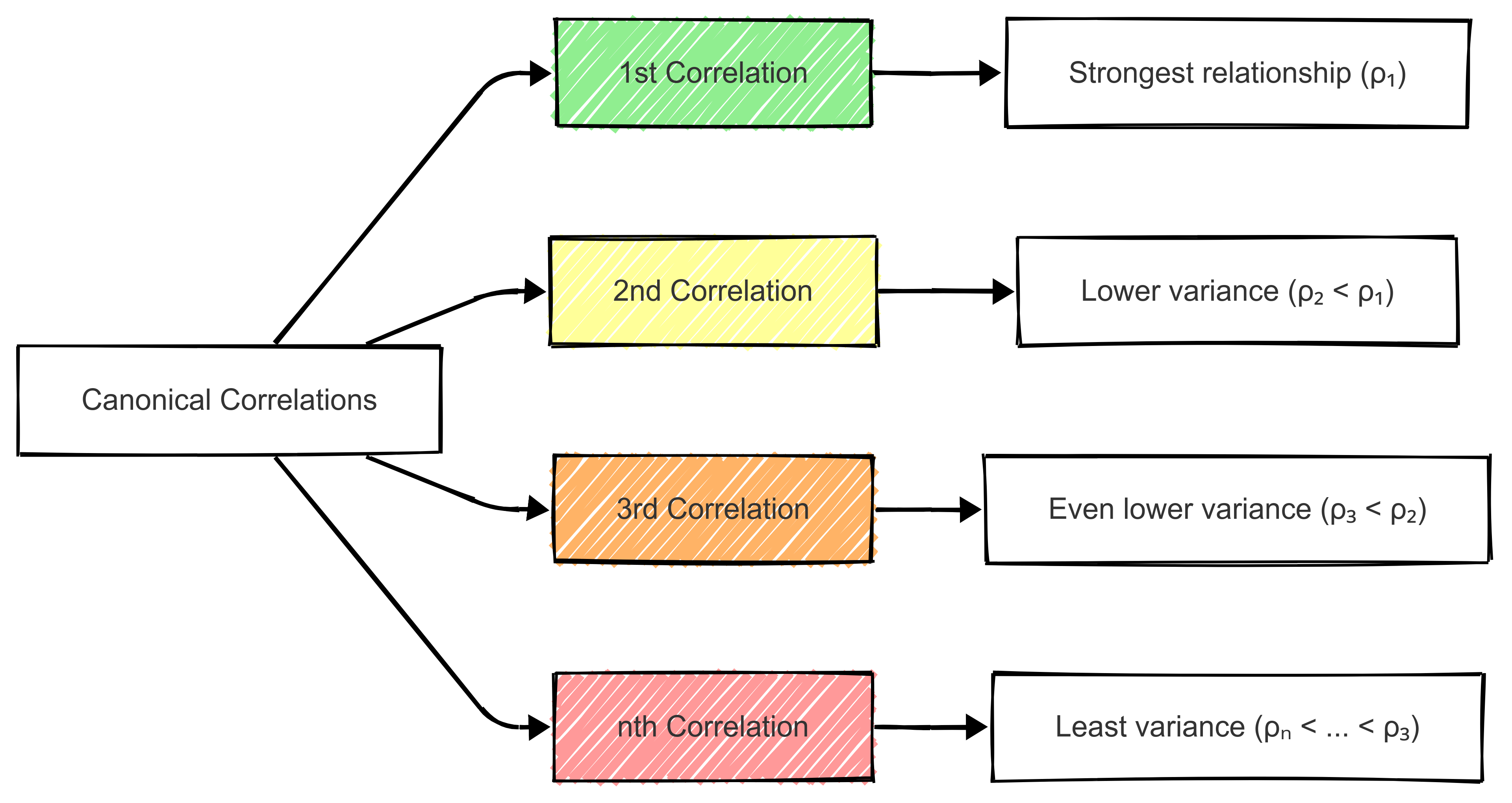
The diagram above illustrates how each successive canonical correlation (ρᵢ) explains less variance than the previous one, with the first correlation capturing the strongest relationship between variable sets.
Decreasing Strength of Canonical Correlations
Therefore, as additional canonical variates are extracted, their explanatory power diminishes.
This means that while the first few canonical correlations may be meaningful, later ones may capture noise rather than substantive relationships. This is important in applications such as sport analytics, where understanding the most influential factors in performance may be more valuable to us than explaining marginal variances.
Limits on the Number of Useful Canonical Variables
The number of meaningful canonical correlations is limited by the smaller of the number of variables in each set. However, not all extracted canonical variables will be useful. In practice, we should assess the statistical significance of each correlation and discard those that do not contribute meaningful insight.
Meaningful Correlations in Sport Analytics
In practice, meaningful canonical correlations can be identified by:
Evaluating the strength of the first few correlations to determine their practical significance.
Assessing the interpretability of the canonical variates, ensuring they align with known performance indicators.
Using significance tests to eliminate weak or redundant correlations.
By focusing on the strongest and most interpretable canonical correlations, we can extract actionable insights, such as identifying key physical attributes that contribute to an athlete’s success.
8.5 Assumptions of CCA
Like any statistical method, CCA relies on assumptions about the data. Meeting these assumptions ensures the validity and reliability of the results.
We have covered these assumptions previously in the module.
- Linearity
- The importance of linear relationships between variables.
- Testing for linearity in CCA.
- Addressing violations of linearity.
- Multivariate Normality
- Explanation of multivariate normality in CCA.
- Assessing and testing for normality.
- Consequences of non-normal data on canonical correlations.
- Independence within Variable Sets
- Assumption of independence among variables within each set.
- Strategies for dealing with highly correlated variables.
- Multicollinearity diagnostics and remedies.
8.6 Applications of CCA
Canonical correlation analysis (CCA) is a versatile technique with numerous applications across different fields.
In this section, we’ll explore three key applications of CCA:
- Exploratory Data Analysis (EDA): CCA can be used to uncover underlying relationships between two sets of variables, providing insight into complex data structures and facilitating hypothesis generation.
- Prediction and Forecasting: By identifying strong associations between variable sets, CCA enables predictive modeling and improves forecasting accuracy in various domains.
- Feature Reduction: CCA helps reduce the dimensionality of datasets by identifying the most informative linear combinations of variables, leading to more efficient data analysis and modeling.
Each of these applications leverages CCA’s ability to handle multivariate relationships.
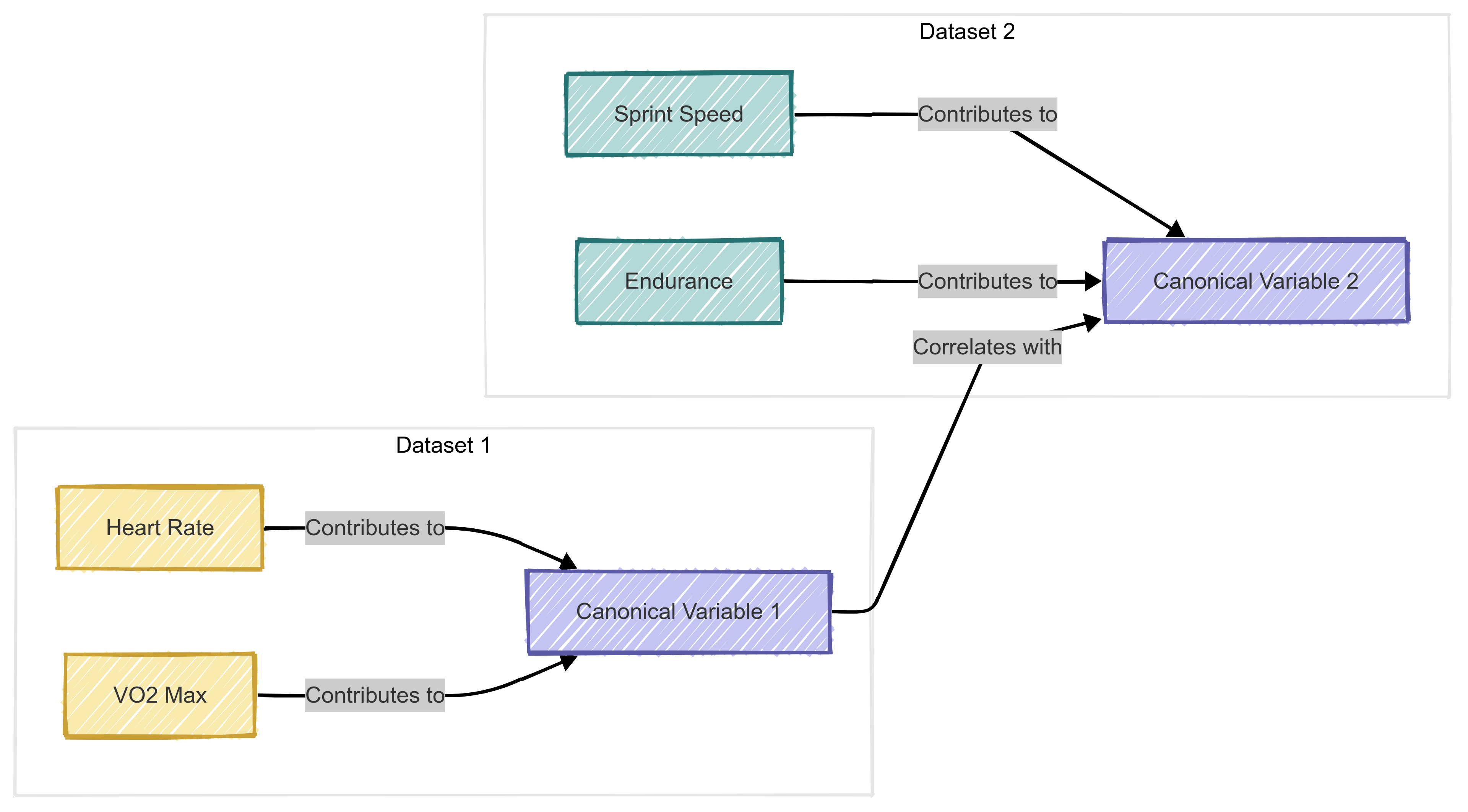
8.6.1 Exploratory data analysis
CCA is widely used in exploratory data analysis to uncover latent relationships between two sets of variables. By identifying canonical correlations, researchers can determine how strongly related the datasets are and which variables contribute most to the relationship.
For example, in sport analytics, CCA could reveal how physiological variables (e.g., heart rate, VO2 max) relate to performance metrics (e.g., sprint speed, endurance).
A high canonical correlation between these sets suggests that changes in physiological measures strongly predict performance.
8.6.2 Prediction and forecasting
CCA is an effective tool for prediction and forecasting because it identifies the strongest associations between two datasets, allowing models to leverage these relationships for better predictions.
For instance, in financial analytics, CCA can be applied to forecast stock prices based on macroeconomic indicators (e.g., inflation, interest rates). By selecting the most predictive canonical variates, analysts can improve their forecasting accuracy.
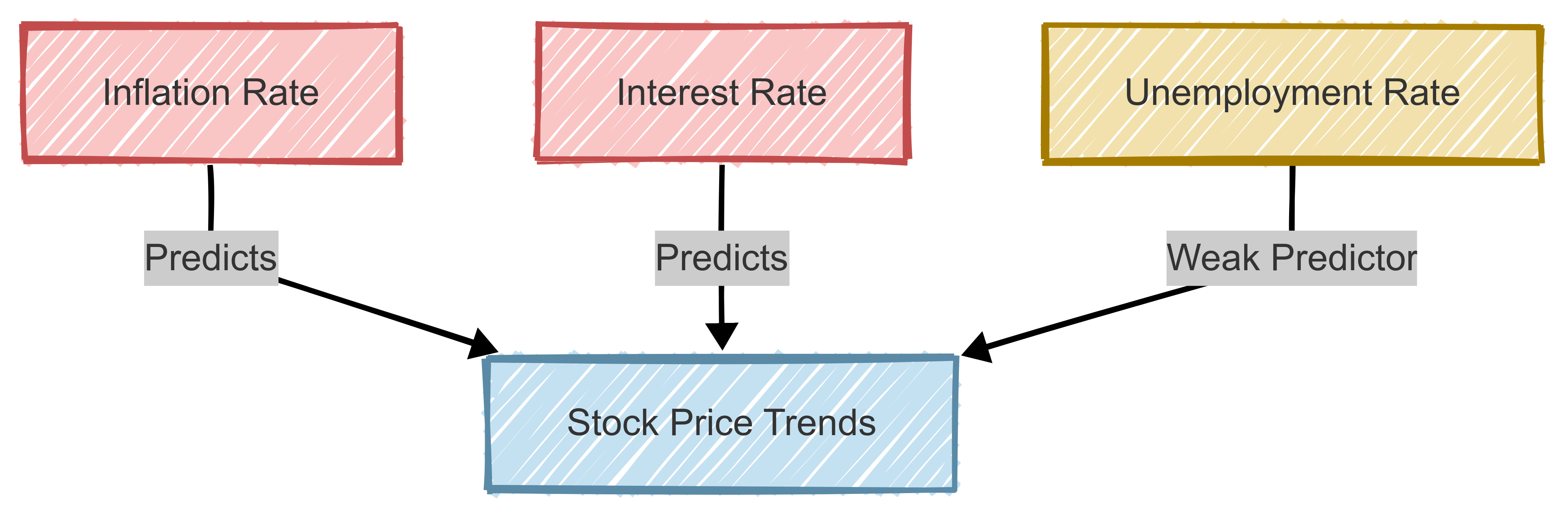
This approach clarifies which economic factors are most influential in stock price forecasting.
8.6.3 Feature reduction
CCA is also useful for reducing the dimensionality of datasets while preserving key relationships between variables,
Instead of analysing a large number of variables independently, CCA identifies meaningful linear combinations that capture the most variance.
For example, in biomedical research, CCA could reduce the number of biomarkers needed for disease prediction by selecting the most informative combinations from a larger set of physiological measures.
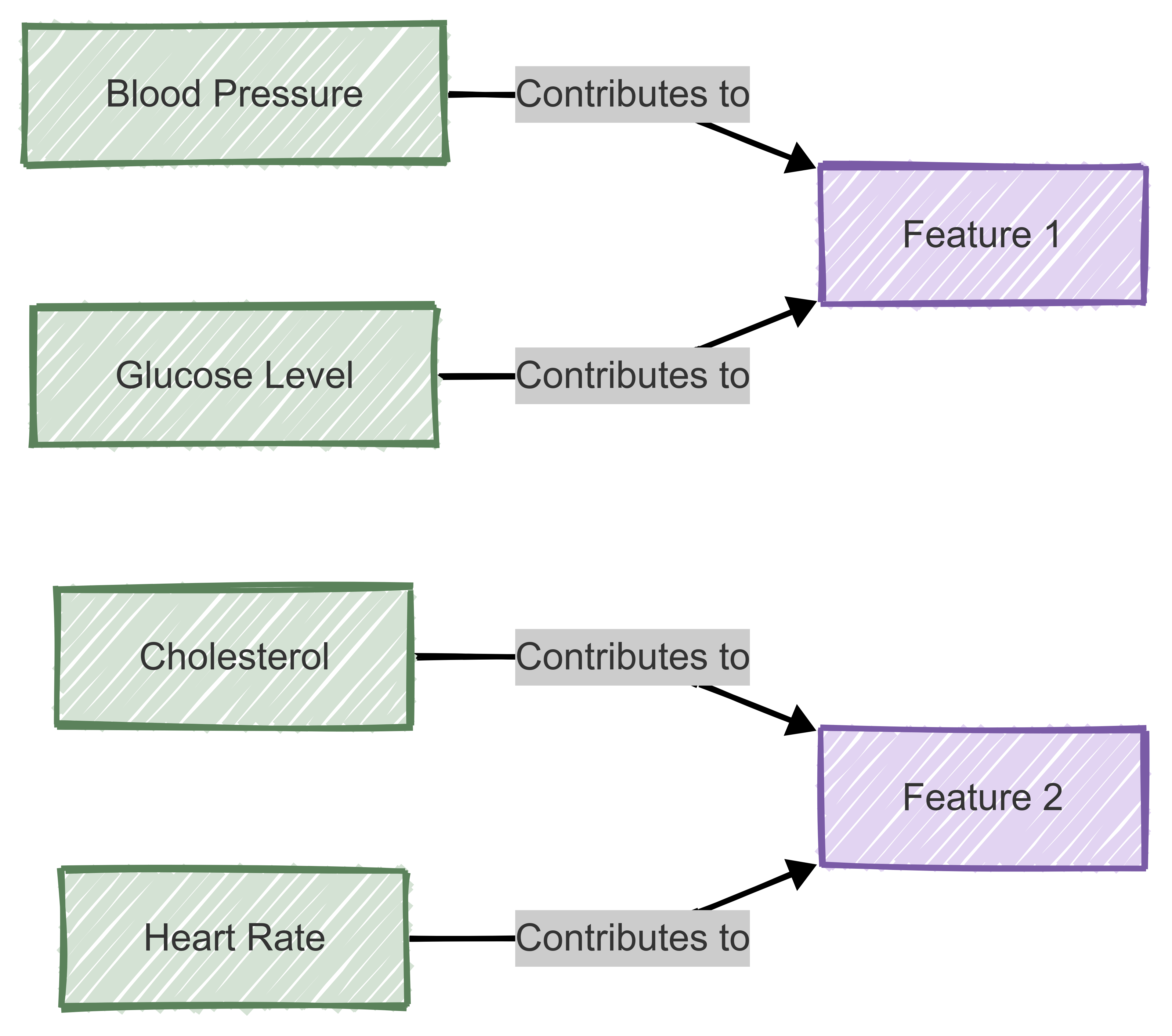
Therefore, by reducing the number of variables while maintaining interpretability, CCA helps streamline analysis and improve model performance.
8.7 Limitations and Extensions of CCA
Despite its usefulness, CCA has several limitations that must be considered when applying it to real-world problems.
For example:
8.7.1 Sensitivity to Outliers
CCA relies on linear relationships between variable sets, making it highly sensitive to outliers. Extreme values can disproportionately affect the canonical correlations, leading to misleading results. Robust statistical techniques, such as data transformation or trimming extreme values, can help mitigate this issue.
8.7.2 Handling Non-Linear Relationships
CCA assumes that the relationship between variable sets is linear. If non-linear associations exist, standard CCA may fail to capture these patterns effectively. Kernel-based CCA and deep learning-based alternatives, such as neural canonical correlation analysis (NCCA), can help model complex, non-linear relationships more accurately.
8.7.3 High-Dimensional Data Challenges
When dealing with high-dimensional data, CCA may suffer from overfitting and numerical instability.
High-dimensional data refers to datasets with a large number of variables (features) relative to the number of observations. This is common in fields such as genomics, image processing, sport analytics, and finance, where hundreds or thousands of measurements might be collected for each subject or event.
Regularised CCA (RCCA) and sparse CCA (SCCA) address these issues by introducing constraints that reduce model complexity and improve interpretability. These methods are particularly useful in applications like genomics and finance, where the number of variables often exceeds the number of observations.
8.7.4 Future Directions
Advances in machine learning and deep learning have led to the development of more flexible variations of CCA. These include:
- Kernel CCA: Uses kernel functions to capture non-linear relationships.
- Sparse CCA: Enforces sparsity to improve model interpretability in high-dimensional datasets.
- Deep CCA: Uses neural networks to learn complex representations and capture hierarchical relationships between datasets.
We won’t cover these in B1705 but they are worth following-up if you’re interested.